

The value of money going to different groups
Posted 2 May, 2017 (updated 25 April, 2023)
It is well known that an extra dollar is worth less when you have more money. This paper describes the way economists typically model that effect, using that to compare the effectiveness of different interventions. It takes remittances as a particular case study.
Assessing the marginal value of an extra dollar
The poorer someone is, the more an extra dollar is worth to them. This effect is often taken into account by economists, particularly when analysing how individuals assess risky situations. However, sometimes it is not accounted for: cost benefit analysis is usually done without distributional weights.
Economists model this effect using a utility function. The utility function defines a relationship between utility (value to the individual) and the individual’s consumption over a given time period. Consumption is the effective amount of money worth of goods and services they use in a year.1 Many different equations have been proposed for the utility function, but one common form is the isoelastic utility function. This equation has one free parameter, known as η (‘eta’, which sounds ‘e’ for ‘elasticity’), which represents how steeply returns to consumption diminish. η must be between 0 and ∞, and can be estimated empirically.
The equation, for utility (u) at a given consumption level (c), and elasticity (η) is:
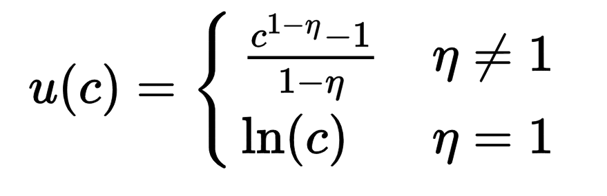
From this it follows that for η = 0 utility is linear in consumption, for η = ½ utility is the square root of consumption, and for η = 1 utility is logarithmic in consumption. Values of η above 1 correspond to utility having a finite upper bound, which is approached hyperbolically as consumption increases.
However, the main use of the equation is to just compare the slope of the curve at one consumption level to the slope at another consumption level. For example the ratio of the slope at $1,000 per annum to the slope at $10,000 per annum shows us the relative value of giving an extra dollar to someone with annual consumption $1,000 versus to someone with $10,000. When performing this calculation, the equation is very simple:
Giving a dollar to someone with k times as much consumption
is worth only (1/k)^η^ times as much.
is worth only (1/k)^η^ times as much.
There have been many attempts to measure η, and it is typically found to be between about 1 and 2. If η equals 1, then we have logarithmic utility of consumption and we have the very simple rule that a dollar is worth 1/k times as much if you are k times richer (and that doubling someone’s income is worth the same amount no matter where they start). If η equals 2, then we have to raise this to the power of 2, so being 10 times richer would mean a dollar is worth just 1/100th as much (and doubling your income is worth much less the higher your starting income). The truth is probably in between these limits. When doing analysis one could pick a preferred value for η and run with that (e.g. η = 1.5), or do a sensitivity analysis by calculating both extremes. I will do the latter.2
Note that if one wants to allocate additional moral value to helping the worse off (i.e. prioritarianism), this can be achieved by increasing η above and beyond the experimentally determined rate (e.g. by adding 1 to it).
Consumption multipliers
Table 1 shows the consumption levels of several different groups of people, alongside numbers representing how much more utility they gain from a marginal dollar compared to the gain for a median US citizen.
| Group | Annual Consumption | η = 1 | η = 2 |
|---|---|---|---|
| Median US income3 | $21,000 | 1× | 1× |
| US poverty line4 | $6,000 | 3.5× | 12× |
| Mean income in Kenya5 | $1,400 | 15× | 230× |
| World Bank’s international poverty line6 | $230 | 91× | 8,300x |
| GiveDirectly’s average recipients7 | $180 | 120× | 14,000× |
| Table 1. Some key consumption levels. |
In Doing Good Better, Will MacAskill talks of the hundred-fold multiplier. This is a rule of thumb that giving money to people living in global poverty does about 100 times as much good as it would in the pocket of someone in a rich country. He considers this to be a baseline for how much good we could expect to do by donation — well targeted donations could get additional leverage on this. This factor of 100 is reflected above by the ratios of 91× and 120× that we see in the bottom two rows (depending on how far below the global poverty line the recipient is). Note that it is only a factor of 100 when η ≈ 1 (which was MacAskill’s conservative assumption). For η = 2, it is a multiplier of about 10,000.8 9
We can also use the ratios from Table 1 to roughly compare the value of programmes to help people living in poverty within a rich country like the US or to help people living in poverty in the poorest countries. The US poverty line is about 25 times higher than the World Bank’s international poverty line. Thus if money was directly given to people at these incomes, one would expect it to go between 25 times (η = 1) and 625 times (η = 2) further if targeted at people in global poverty. Any particular intervention might be better or worse than a cash transfer by some leverage factor, but if we have no reason to believe these factors are generally higher for one type of poverty than the other, then this ratio is unchanged. And if we do have some information about which has higher leverage, this is simple to incorporate.
This approach is very general, and can be used in many different types of impact evaluation. For instance, it could be used to compare the additional value of targeting the poorest people in a country rather than the median (showing you how to balance this advantage against the additional costs of that targeting). These ratios can also be used to adjust unweighted cost-benefit analysis: weighting each person’s willingness to pay by the relevant multiplier.
Leverage
Sometimes non-monetary interventions can help an individual more than a simple monetary transfer. The ‘leverage’ of a particular intervention is its benefit-cost ratio, where benefits are assessed in monetary equivalents for a particular group. If the leverage of an intervention is greater than one, then it outperforms a monetary transfer to the affected individuals. Note that the idea of leverage is only defined relative to a particular income level.
A particular case of examining leverage comes from an exercise done by GiveWell where its staff tried to judge the relative value of donating a dollar to GiveDirectly to that of donating a dollar to the Against Malaria Foundation (AMF). The median estimate was that the AMF programme does about 2.2 times as much good per dollar, whilst the highest estimate was that AMF is 13 times more effective.10 This suggests that AMF’s leverage is around 2.2. Various meta-charities have also compared their effectiveness to that of the charities they (directly or indirectly) raise for, since they are able to leverage donations to them by encouraging effective giving. Several such effectiveness estimates are summarised in the table below, although we should highlight that these estimates may not be very robust.11
| Charity | Relative effectiveness |
|---|---|
| GiveDirectly | 1× |
| Against Malaria Foundation (median estimate) | 2.2x |
| GWWC (already donated to top charities)12 | 6x |
| The Life You Can Save13 | 9x |
| Against Malaria Foundation (highest estimate) | 13x |
| Raising for Effective Giving (2016 average fundraising ratio)14 | 17x |
Table 2. Various rough estimates of relative effectiveness of some key charities.
So far we have introduced the idea of an income multiplier (as shown in Table 1) and a leverage ratio (as shown in Table 2). We can now combine these ideas. The value of a dollar to a particular intervention (relative to some baseline) is simply the consumption multiplier for the group it affects, multiplied by the leverage ratio of that particular intervention. So effectiveness is consumption multiplier multiplied by leverage ratio.
We can now apply this to make comparisons between things on both tables: A dollar to GiveDirectly is roughly the same as a dollar to the typical person it serves (~90% of donations go through to recipients, and assuming that there is not too much variation in the consumption level of recipients). Now, we can use the fact that relative effectiveness is leverage multiplied by consumption multiplier. A dollar to AMF is worth 10 times that of a dollar to GiveDirectly, which, on the assumption of η=1, is worth at least 120 times as much as a dollar in the pocket of a person at the US median income. Therefore, that dollar would create ~1,200 times as much value if donated to AMF (a hundredfold multiplier with a tenfold leverage).
Case study: remittances
Remittances are transfers of money from foreign-born workers to people in their home country. The sort of analysis used above can also help us think about the importance of making remittances more effective.
Table 3 shows the scale of some important global expenditures.
| Group | Annual Spend |
|---|---|
| Global Fund15 | $4 b |
| DFID health spending16 | $3.5 b |
| DFID total spending17 | $14 b |
| Total Aid18 | $160 b |
| Total remittances19 | $436 b |
Table 3. Some key annual expenditures.
Many have noted that remittances dwarf all Aid — at least in terms of the raw size of the monetary flow. Should individuals (and groups like GiveWell and Giving What We Can) focus more on them? We can use the earlier results to help with this. I don’t know of any good figures for the consumption distribution of remittance recipients, but would be surprised if the relevant average (which is not the arithmetic mean20) were less than 10 times the consumption level of GiveDirectly recipients. If so, then the total of remittances is worth the same as about $4 billion to $40 billion allocated through GiveDirectly.
Thus, since total aid spending is around $160 billion, the mean value of aid dollars only needs to be something like 2.5% or 25% that of GiveDirectly for the value of aid to outweigh that of remittances. It seems likely that aid spending meets this bar, particularly since total aid spending includes a substantial amount of money on things that are much more effective than GiveDirectly. As an example, even just the $4 billion of Aid that goes on the Global Fund only needs to be 1 or 10 times as effective as GiveDirectly to outweigh remittances. Therefore, it seems likely that total aid spending is worth at least as much as remittances are.
We could also evaluate the size of the benefit we could get by improving remittances, such as by eliminating remittance fees. The average cost of sending back remittances is about 8%. Thus, about $34 billion per year are lost to the poor in transaction fees which could theoretically be reduced to near zero. Let us again assume the relevant income average of remittance is recipients is ~10 times that of GiveDirectly recipients. According to this estimate, the amount currently wasted in transaction fees is worth something like $340 million to $3.4 billion to GiveDirectly per annum: a very large amount, but smaller than it might initially have appeared.
Footnotes
- While income is what you earn, consumption is what you spend. It is generally regarded as more relevant for determining the utility of one’s money, since it includes things like home grown food or spending of saved money and excludes things like adding to one’s savings. In the absence of data on consumption, income is often used as a proxy. ↩
- Note that if you are uncertain over a variety of values for η, higher values of η will dominate the analysis, since they give more extreme results. ↩
- Median household income in 2014 was $53,657 and I have divided by the mean family size of 2.54. ↩
- The line depends on the family composition. This is the 2016 rate for a family of 4. ↩
- GDP per capita at official exchange rate, 2015 estimate from CIA World Factbook. ↩
- As of 2015, this was $1.90 per day in PPP terms. I have assumed an average PPP rate of 3, to turn this into $0.63 per day in official exchange rate terms. ↩
- http://www.givewell.org/charities/give-directly#footnoteref145_r2lrnsl. Note that only 90% of the money gets to the recipients, so if considering the value of a dollar given to GiveDirectly rather than to its recipients, then these factors should be multiplied by 0.9. ↩
- That this figure is so high, perhaps implausibly high, gives us some reason to doubt that η = 2. ↩
- Interestingly, purchasing power parity adjustments don’t come into this. A dollar to someone at the global poverty line is about 100 times as valuable as to the typical US citizen because it increases the poor person’s consumption by about 100 times as high a proportion (i.e. by 0.5% vs 0.005%), not because it will be able to buy about 3 times as much rice in Kenya as it can in the US. A dollar given to a Kenyan will go further than one given to an American. But the Kenyan person’s initial money was also going further (so they are further along on the consumption curve). In terms of who benefits more from the extra dollar, these effects cancel out. Therefore, it isn’t more important to help someone living on $200 per year (at official exchange rates) in a place where PPP is high than someone on the same amount where PPP is low. We thus want all of our units to stay in official exchange rate terms. Note that a correction to this footnote was posted on the EA Forum in March 2023. ↩
- See their cost-effectiveness analyses: http://www.givewell.org/how-we-work/our-criteria/cost-effectiveness/cost-effectiveness-models Elie Hassenfeld’s estimate is slightly lower, and other staff members give a wide variety of different estimates. ↩
- NB also that these figures assume that the average effectiveness of donations tracked by these meta-charities is equal to the GiveDirectly’s effectiveness: in reality, many of the donations were to the Against Malaria Foundation and other charities that may be more effective than GiveDirectly, so the relative effectiveness estimates for the meta-charities may be underestimates. A full assessment would include an assessment of the meta-charities true leverage ratio, and assessments of the efficacy of all of the charities they diverted funds to. ↩
- Estimate for 2017. ↩
- In 2013. ↩
- 2016 budget. ↩
- ODA in 2013. ↩
- In 2014. ↩
- The relevant average is somewhat complicated. If η = 1, we should use the harmonic mean. Note in particular that not only the arithmetic mean, but also the distribution of consumption values should be accounted for. ↩
- University of Oxford. Thank you to Max Dalton, Michelle Hutchinson, Owen Cotton-Barratt, Rob Wiblin, and Ben Todd for helpful comments. ↩