Defining returns functions and funding gaps

As organisations receive more funding, the value of extra funding changes. This is relevant for donation decisions. People have used various concepts to discuss this feature:

• Room for more funding
• Funding gaps
• Diminishing (marginal) returns

I want to dig into what people mean when they use these terms.

I ground these terms by distinguishing between two families of models: returns functions and funding gaps. It is usually best to be explicit about which model you are using.

True returns

Every dollar an organisation receives has some impact, which I will call the ‘true returns’ to additional funding. Impact as a function of funding might look like Figure 1 below.^fn-2 If we could observe these true returns, we would be able to know the impact of an additional dollar when $X have already been donated. It is simply the slope of the true returns curve at $X.

Figure 1

However, the true returns curve is normally impossible to observe directly, and often too complicated to use even if we could observe it. We therefore have to use models which incorporate our uncertainty. Thus when we talk about the returns to funding, we are normally discussing some model of the true returns, rather than the true returns.

Models of true returns

Normally, the returns from additional funding diminish in expectation beyond a certain point. One concept which implicitly appeals to this fact is funding gap (sometimes called room for more funding). It is based on the assumption that that funding is significantly less impactful (or not impactful at all) beyond a particular point.

The other main approach instead specifies some returns function of how impact increases with donations.

These approaches are closely related: indeed, funding gap models could be seen as a special type of returns function model. However, funding gaps, unlike returns functions, emphasise that there is an optimal level of funding. In what follows, I will set out the two approaches and explain how they relate to each other.

Returns functions

Returns functions specify a functional relationship between an organisation’s funding and its expected impact.^fn-3

Two desirable features of returns functions are:

1. Closeness of fit: The function should match our evidence about what true returns look like. In practice this normally means:

   1. Increasing: The function should be non-decreasing, since additional funding normally don’t reduce the impact of the organisation, and generally increases it (at least in expectation).
   2. Concavity****: The function should be concave, since it is normally assumed that as total funding increases, each additional dollar provides slightly less impact than the last. This is empirically supported, but also what we expect theoretically if organisations take their most cost-effective opportunities first.

2. Clarity: The form chosen should be easy to use and understand. One tenet of clarity is:

   1. Simplicity: Simpler functions are easy to use and understand

Some functional forms are particularly common:

Logarithmic returns function

One common form is the logarithmic relationship, y=a + logb(x). This form appears to be a good approximation for returns in areas such as research, and there are also some theoretical reasons to expect this functional form. This form also has some properties that make analysis easier.

Figure 1

Root returns function

Another common form is to have impact related to some root of x: , where b>1 so that returns are positive but decreasing. Again, this functional form is easy to use.

Holden Karnofsky writes “I might roughly quantify my intuition by saying that (at the relevant margin) giving 10x as much would only accomplish about 2x as much.” If we extrapolate this idea to a range of scales, this implies a root function, where b=log2(10)~=3.3.^fn-6

Piecewise linear

With a piecewise linear function, impact is a linear function of funding, but the slope coefficient is different for different ranges of x. For instance:

y=a +bx for 0<x<c

y=d + ex for x>=c

If returns are increasing and concave, b and e are positive, with b>e. We might instead have multiple slope changes. These linear functions are easy to explain to less technical audiences.

Figure 3

Funding gaps

The ‘funding gap’ notion emphasizes that organisations should not be funded beyond a certain point. A literal or strict interpretation of the term ‘funding gap’ may suggest that organisations produce no value beyond a certain funding level. However, this strict view seems so harsh that I suspect that no-one believes it. A more plausible interpretation assumes that there are other charities that one can give to. The presence of these outside options implies that there is an optimum funding level for each organisation. We may define a weaker notion of a funding gap based on that idea.

Strict funding gap models

On the strict funding gap approach the returns curve is flat beyond some value, $X*. Now the strict funding gap is defined as the amount that the charity could usefully spend ($X*), minus the amount of funding it has received to date ($X).

This model is a special case of the returns function approach, where the returns curve is flat beyond a certain level of funding. But this upper bound on impact generates an important feature, namely that there is a clear optimum funding level $X*. Since $X* is clearly defined, the funding gap is X*-X.

Figure 4

This model is the most literal and naive interpretation of the term, so it is worth setting it out, alongside more plausible funding gap models.

Relative funding gaps

Suppose there is some clear alternative option for buying impact: the ‘next best’ giving opportunity. Call the social return (impact) per $ of donation to this alternative the ‘relative price’—since optimal funding decisions are made relative to this alternative.^fn-7   Given the other opportunities available, we should fund the organization when that is the cheapest alternative, and cease funding it when other opportunities are cheaper. This implies that, in the figure below, it is optimal to fund the charity to the level of exactly $X*.

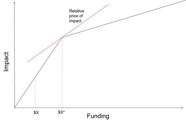Figure 5

Note that the returns function is identical to that in Figure 3 above. The difference is not in the shape of the returns function, but in the fact that there is a price that the donor is willing to pay for impact.

Since it is optimal to fund the charity to level $X*, it makes sense to speak of a ‘relative funding gap’ equal to the difference between the optimal funding level given the relative price, and the current funding level.

However, this funding gap is not absolute, as in the strict funding gap model: if the relative price changes, so will the relative funding gap. Therefore, the funding gap of one organization may change if another organization gets more competitive, or if the amount of funding to other organisations increases. In particular, if the returns curve is strictly concave, then if the relative price decreases (more impact per marginal $), the relative funding gap will decrease. If the relative price increases (less impact per marginal $), the relative funding gap will increase. This is shown in figure 6:

Figure 6

Despite this difference, both strict and relative funding gap models imply that there is some level beyond which the organisation should not be funded.

Robust relative funding gaps

Suppose instead that there is some inflection point in the returns function: some point beyond which, returns diminish steeply, but do not disappear. Figure 7 shows such a returns curve. Since there is an inflection point at $X*, then for many different prices, including the three prices shown, $X* is the optimal amount of funding for this charity. We might say that $X* is the robust optimal amount of funding for this charity, and so that $X* - $X is the robust relative funding gap.

Figure 7

Note that for some prices, $X* is not the optimal level of funding, so unlike in the strict model, the funding gap depends on the efficiency of alternatives. However, unlike the relative model, the funding gap is somewhat resilient to changes in the efficiency of alternatives.

The relationship between returns functions and funding gaps

The relationship between these families of models is somewhat nuanced.

In one sense, the funding gaps models are a special cases of returns functions models, since they are based on returns functions. On this view, funding gaps models are simply special returns functions with a particular clear inflection point, beyond which returns diminish steeply. This implies that the difference between funding gaps and returns functions is simply a matter of degree. This is certainly one aspect of the difference between the models: funding gaps models normally have more of an inflection point than returns functions do.

However, plausibly funding gaps models are more than just a special case. By explicitly noting the presence of alternative organisations (or an upper bound on returns in the case of the strict model), they reach a different practical conclusion: that there is some upper bound on how much funding organisations should receive. Funding gaps say something about the optimal funding level for the organisation. Whilst returns functions could imply optimal funding levels, they don’t make the additional assumptions needed to do so, so their import is different. This greater prescriptivity of funding gaps models makes them a different kind of model than returns functions, rather than simply a special case.

Other/hybrid models

GiveWell use a model that appears to be some hybrid between these two accounts. In particular, they appear to use something like the strict funding gaps model, but with uncertainty over the size of the funding gap, which means that the expected value of funds diminishes as it becomes more likely that the gap has been filled. This can therefore either be viewed as some form of probabilistic funding gap model, or as a concave returns function in expected value.

There may be other hybrid models, or even totally different approaches to modeling diminishing returns, that I am not aware of, or that have not yet been invented.

Concluding discussion

Thinking explicitly about what we mean by ‘returns curves’ and ‘funding gaps’ should allow researchers to be clearer about how they are modelling  true returns. Also, by explicitly acknowledging the variety of possible models, we highlight that ‘funding gap’ and ‘logarithmic returns’ are concepts used to talk about models of reality, rather than reality itself.

Explicitly stating which model you are using allows you to communicate with less ambiguity. There are costs to being so explicit: it involves using more formal language, and may be offputting to a general readership. However, in general it seems better to be explicit about the way you’re modelling diminishing returns, and be explicit that you are only discussing a model of reality.

The second post in this series will discuss how to select the best model for different returns, and will argue that returns functions are generally preferable to funding gaps.^fn-1

---